How Much Is a Hundred Bucks?
The not so mobile-friendly calculator accompanying this post can be found here.
The value of time, the value of money
There are various ways of trying to assess the value of something. For instance, one might define the value of a resource by how much someone else is willing to pay for it. In the domain of time, we could ask the question of the hourly rate someone is willing to pay for our time/labor and consider that the value of our time.
A contractor or employee might be able to gauge how much other people are willing to pay for an hour of their time and derive from that an aspirational hourly rate, as suggested by Naval. In this mindset, one might take on the stance of never ‘doing work’1, e.g. filing taxes or doing laundry, which costs (framed differently, ‘pays’) less than said aspirational hourly rate. The implicit assumption here is that work and time are fairly liquid resources - instead of cooking a meal for an hour we could decide to do an additional hour of some work which pays best and keep the difference.
Since this is a voluntary trade, we assume it was fair/efficient and think of both resources having equivalent value. Hence, the hourly rate, defining the value of time in terms of money, would also imply a valuation of money in terms of time.
While this view might be useful in many regards, it doesn’t perfectly capture what I want it to capture.
On the one hand, it doesn’t explicitly2 account for temporal developments, such as returns on investment over the years. For example, a dollar saved now might be ‘more valuable’ in terms of time gains than a dollar saved in ten years, depending on (compounding) returns on investment and depending on one’s capability to increase hourly pay over the years.
On the other hand, the previous view relies on the assumption that we can and would trade time for money until the end of one’s days.
What seems more natural for me to do is to emphasize that, in a very simplified model of employment, one is renting out one’s time until ones doesn’t ’need’ to anymore - ideally hoping that this is strictly before the moment a respective national pension fund kicks in. After that point in time, one might still go after the very same activity but with a very different motivation: no longer trading time for money but rather just allocating time on what’s best fun, most exciting, most rewarding. In this model, the monetary unit remains the same as before: the typical currency, say USD. Yet, the temporal unit changes: it is no longer an hour of one’s time ‘right now’ but rather the delay from achieving financial independence that a monetary unit causes.
Bluntly put, the cost model for money becomes: By how much does spending a given amount delay the point in time of reaching the bliss of financial independence?
Note that the answer to this question doesn’t change whether one continues to receive income from employment or contracting after this point in time. This is a relevant since we are talking about financial freedom, in a somewhat stark contrast to retirement. Also note that this approach assigns value to one’s time in a way that immediately factors in cost of living. In contrast, the former, aspirational hourly wage model didn’t. For example, deciding not to trade one hour of one’s time for money leaves it open as to how the bills are paid.
In this alternative cost model it is clear that the more we spend before reaching our savings goal, the longer it’ll take us to reach it. Put differently, the less we spend, the more time in a state of choice, of freedom, we earned ourselves. But how much time? We’ll get to that in the next paragraph.
Moreover, we will realize that the respective values of time and money are likely to change over time.
How much is 100 USD, formally?
How much do we save?
Let’s say that
- The annual savings as of now are $s$, e.g. 50,000 USD.
- The annual savings increase every year by $\rho_s$, e.g. 0.07.
- There is a fixed annual return on savings investments of $\rho_i$, e.g. 0.04.
- There is a savings goal $g$, e.g. 1,000,000 USD. One might define this as the yearly spending divided by $\rho_i$ minus current savings.
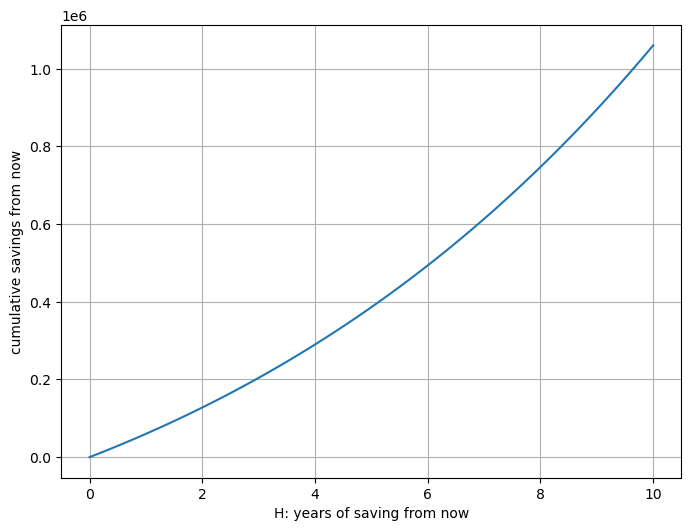
Under these assumptions, the cumulative savings after $H$ years equal:
| $H$ | Savings after $H$ years |
|---|---|
| 0 | 0 |
| 1 | $s$ |
| 2 | $s(1+\rho_s) + s(1 + \rho_i) \\ = s[(1+\rho_s) + (1+\rho_i)]$ |
| 3 | $s(1+\rho_s)^2 + s(1+\rho_s)(1+\rho_i) + s(1+\rho_i)^2 \\ =s[(1 + \rho_s)^2 + (1 +\rho_s)(1 + \rho_i) + (1 + \rho_i)^2]$ |
It can easily be shown by induction that this series equals the following expression, which can be further simplified:
$$ \begin{aligned} f(H) &= \sum_{y=0}^{H-1} s (1 + \rho_s)^y (1 + \rho_i)^{H-1-y} \\ &= s (1 + \rho_i)^{H-1} \sum_{y=0}^{H-1} \left(\frac{1 + \rho_s}{1 + \rho_i} \right)^y \\ &= s (1 + \rho_i)^{H-1} \frac{1 - \left(\frac{1 + \rho_s}{1 + \rho_i} \right)^{H}}{1 - \frac{1 + \rho_s}{1 + \rho_i}} \\ &= s (1 + \rho_i)^{H} \frac{1 - \left(\frac{1 + \rho_s}{1 + \rho_i} \right)^{H}}{\rho_i - \rho_s} \\ &= \frac{s}{\rho_i - \rho_s} [(1 + \rho_i)^{H} - (1 + \rho_s)^{H}] \end{aligned} $$
Here we used the sum formula of the geometric series. In other words, we assumed that $|\frac{1 + \rho_s}{1 + \rho_i}| \neq 1$. Hence, we assume that $\rho_s \neq \rho_i$. If they were equal, we could apply the formula for the geometric series, too, simply to a different, more simple summation term.
The following plot shows the function $f$ from above for varying time horizons $H$ and some arbitrary parameters $s$, $\rho_i$ and $\rho_s$:
We could now subtract the savings goal from this function and try to find the root of that expression, with respect to $H$. This is an expression of the form $a^H + b^H - c = 0$. As far as I can tell3 there are, in the general as well as this very case, no analytical solutions for such expressions. As a consequence we can’t easily invert the function from above and can’t have a mapping from cumulative savings to duration of saving.
Still, what we can do is to try to numerically look for the duration which yields a certain cumulative saving. Put differently, we can tackle the following problem:
Find the $H$ such that $f(H) = g$
This can be achieved by looking for the root of $f(H) - g$ with the Newton-Raphson method.
In summary, we have a way of determining the duration of saving $H$, given a savings goal $g$.
Having figured out how much we save in a given duration and how long we need to save for a given savings goal if all goes according to plan, let us now continue this exercise, taking additional expenditures into account.
How much is 100 USD in USD?
In the previous paragraph, we illustrated how savings from now will compound. Spending a sum of money now, will - in a sense - also compound, since we are missing out on the return on investment had we not spent but invested this money.
Gladly, this compounding is of a simpler nature than that of the savings. The savings came with two interdependent compounding aspects: the return on investment as well as the increase in annual savings. For an expense $e$ made right now, there is only the return on investment that is compounding:
$$ \begin{aligned} c(H, \rho_i, e) &= e (1 + \rho_i)^{H} \end{aligned} $$
For example, if we expect to hit our savings goal in $H=10$ years, and we assume an annual return on invest $\rho_i=.05$, spending $e=100$ USD now will ‘cost us’ approximately 163 USD. Put differently, we need to increase our savings goal by 163 USD if we want to spend 100 USD right now.
Importantly, we see that the missed savings potential due to additional expenditures is a monotonically increasing function of the horizon $H$. Put differently, spending 100 USD at time step $t$ is more expensive than spending 100 USD at time step $t + \epsilon$.
How much is 100 USD in time?
We can now tie both previous pieces together. We know how much we save not considering additional expenditures and how an expenditure impacts our savings. In order to figure out for how long we need to save given additional expenditures, we can postulate that our achieved savings disregarding additional expenditures $f(…)$ minus the missed savings potential $c(…)$ should be equal the savings goal $g$.
$$ f(H) - c(H, e) = g$$
As before, we can use Newton Raphson to solve this equation, figuring out for which $H$ this equation holds true. Put differently, we can figure out for how long we need to save taking this expenditure into account.
Comparing this duration with the duration without the additional expenditure then yields the extra time of saving we need to put in.
$$ \begin{aligned} g &= f(H) - c(H, e) \\ g &= f(H’) \\ \Delta &= H’ - H \end{aligned}$$
For example, if our savings goal from now on is $g = 1,000,000$ USD, our annual savings in the next 12 months equal to $s = 60,000$, the annual savings increase $\rho_s = .07$ and the annual return on investment $\rho_i = .05$, spending an extra $e = 100$ USD right now will delay the point by when we reach financial freedom - i.e. ‘it’ll cost us’ - .35 days.
Okay, so we learned that
- Money now will be worth more money later.
- How much time money right now will save us at the end of our time in serfdom.
This bares the question:
How much is 100 USD in time, other than at ’the end’ of our saving period?
In the previous thought experiments we determined the value or cost of 100 USD by framing it as an additional expenditure, moving our savings goal further away. Flipped the other way around, we might ask the question of the value of a 100 USD bill we find on the street with respect to time.
The monetary return on investment will be the same - assuming parameters as in the example above, this will yield 163 USD down the line.
Yet, If we now ask the question of how much time we ‘gain’ the answer might vary. If we seek to simply seek shorten the duration of saving - i.e. removing the time ‘from the end’ - the answer will remain more or less the same - modulo some slight asymmetry. But what if we are now considering to ’take off’ some time somewhen between now and the reaching of financial freedom? Is 100 USD worth the same amount of time at time step $t$ than at $t + \epsilon?
No. But let’s approach this one step at a time. Let’s first ask the question of how much we save when taking a break from earning money of duration $\epsilon_t$ at an arbitrary point in time $t$ between the start and end of saving $H$. In order to answer this question, we can reuse $f$ from before and our savings period into in three sub-phases:
| Phase | time index | Savings produces in this phase |
|---|---|---|
| Pre-break | $0$ to $t$ | $f(t)$ |
| Break | $H_{b}$ to $t + \epsilon_t$ | $b=f(t)(-1 + (1 + \rho_i)^{\epsilon_t}) - \epsilon_t z$ |
| Post-break | $t + \epsilon_t$ to $H$ | $f(H-t, s=s’) + (f(t) + b)(-1 + (1 + \rho_i)^{H-t-\epsilon_t}) $ |
where $s’= s (1 + \rho_s)^{t}$ is the annual saving at time $t$ or $t + \epsilon$[^4] and $z$ is the annual cost of living in USD.
Let’s now add up the savings from each of these phases and simplify:
$$ \begin{aligned} f(t) + b &= f(t)(1 + \rho_i)^{\epsilon_t}) -\epsilon_t z \\ (f(t) + b) (1 + \rho_i)^{H - t - \epsilon_t} &= f(t)(1+\rho_i)^{H - t} - \epsilon_t z (1 + \rho_i)^{H - t - \epsilon_t}\\ f_b(H, t, \epsilon_t) &= f(H-t, s=s’) + f(t)(1+\rho_i)^{H - t} - \epsilon_t z (1 + \rho_i)^{H - t - \epsilon_t} \\ &= f(H-t, s=s’) + f(t)(1+\rho_i)^{H - t} - c(H-t-\epsilon, \rho_i, \epsilon_t z) \end{aligned} $$
Let’s dissect this expression intuitively. The first term basically boils down to our usual savings computation for the duration that is left after the break. What’s special is that we use an updated annual savings number
- since we have already made a career up until our beak at time $t$. Our salary and therefore our annual saving have increased.
The second term expresses that we have made our usual savings $f(t)$ in the pre-break phase - yet, these savings further compounded thanks to investing. The remaining duration of compounding covers the break as well as the post-break phase, hence it amounts to $H - t$ in total.
The third term corresponds to the life costs we had to pay during our break. These had to be paid somehow. We simply frame this as though they had been paid from the then-existing savings. Diminishing the savings at time $t$ means that we lose out on some compounding of these savings. We capture this by directly compounding the life costs, a negative number. We observe that this is the same paradigm as when we wondered about the compounding cost of a 100 USD spending. Therefore we can reuse the function $c$, just with an adapted duration $H - t - \epsilon$ - assuming that the life costs of the break are paid at the end of the break.
Now that we know how much we save even when taking a break at a specific point in time and of a specific duration, we work in reverse and figure out how long a break can be given all other information. Formally, we already found the horizon $H$ leading us to our savings goal $g$. We now ask the question
For a given ‘break moment’ $t$, for how long can we take time off to still meet our savings goal given that just found 100 USD?
This can be answered - who would’ve guessed it - by framing it as an equation that we’ll solve with Newton Raphson.
Find $\epsilon_t$ such that $f(H) - f_b(H, t, \epsilon_t) = c(H, \rho_i, 100)$.
Note that since we found the 100 USD now, they will - since we will of course invest them - compound over the entire time horizon. Therefore we reuse the compounding function $c$ from before.
The following graph show solutions $\epsilon_t$ on the y-axis for varying $t$ on the x-axis. The $H$ was chosen as … in order to produce savings $g=…$.
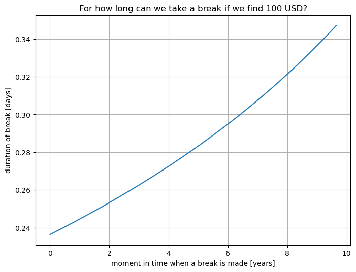
We notice that the duration of time we can take off increases with the delay with which the time off is taken.
A tl;dr for those who did r, a.k.a ’the summary’
First, we learned how much savings we generate after a given amount of years. In order to do so, we relied on a couple of assumptions:
- We currently save a certain amount of money, of which we invest all.
- These investments compound with a fixed annual net return on investment ratio.
- Moreover, the annual savings amount increases with a fixed ratio.
Using this knowledge, we figured out the inverse: for how long we need to save given that we want to reach a certain savings goal. This goal could, for instance represent enough money such that one no longer relies on income from employment to sustain one’s life.
With that knowledge we tackled several questions:
- For how much longer will we need to save if we spend 100 unaccounted for USD right now? (e.g. .35 days)
- By how much do we need to increase our savings goal if we spend 100 unaccounted for USD right now? (e.g. 160 USD)
- How much time could we ’take off from saving’ (e.g. not work in employment) an at an arbitrary moment in time if we found 100 unaccounted for USD on the street right now? (e.g. .24 days right now, 0.28 days in 5 years and .35 days in 10 years, just before reaching our savings goal).
Lastly, one could of course ask the question of how much time is worth in some other moment’s time. Maybe some other time.
I suppose that ‘doing work’ here means anything that takes time and is not substantially intrisically rewarding. Flipped around, this might mean that an employment activity might not necessarily be ‘doing work’. ↩︎
One can of course bake anything into an hourly rate and make define it relative to a point in time - this would then implicitly capture temporal developments. ↩︎
Based on myself not finding a solution, WolframAlpha not finding a solution (something something absence of evidence isn’t evidence of absence) and ChatGPT claiming that this cannot be solved analytically. Sadly I didn’t find a proof for why this can’t be solved. So, I don’t really know. [^4] We assume that we don’t move forward to a raise while taking a break. ↩︎