Markov Random Field Image Denoising

This post describes the application of a Probabilistic Graphical Model for simple image denoising, as suggested in Bishop’s chapter 8.3.8. I will attempt to introduce some notions for general context without derivations. Googling will lead to plenty of useful resources. On an introductory level, I enjoyed Daphne Koller’s class.

Context: Probabilistic Graphical Models

Probabilistic Graphical Models are tools to model and express conditional independencies among a set of random variables.

Why care about conditional independencies? Joint distributions can always be expressed without conditional independencies. Yet, the latter allow for an expression of the joint distribution requiring fewer parameters.

There are two major variants of Graphical Models. Some rely on directed graphs and use the notion of ’d-separation’ for expressing conditional independencies. While there are quite a few flavors of directed Graphical Models, Bayesian Networks are the ones I have encountered most. Another major variant are undirected Graphical Models. A prominent representative of the latter group are ‘Markov Random Fields’, or ‘MRF’ in short.

In Bayesian Networks, nodes of the graph, also called ‘factors’ have a direct probabilistic interpretation: they represent conditional probabilities. In MRFs, the interpretation is less straight-forward; more on that later. Some more information about the relation between directed and undirected models:

• Any directed graph model can be turned into an undirected graph model via a process called ‘moralization’. It consists of ‘marrying’ parent nodes. This process might remove some conditional independencies.
• In general, directed and undirected graph models can capture different conditional independencies; see the next section for more detail.

Remember than any joint distribution can be expressed without the help of conditional independencies. This approach to leads to fully connected graph in Graphical Models.

Maps

Having introduced the notions of both directed and undirected Graphical Models for representing joint distribution, the question of how they relate arises naturally. This question is as interesting as (comparably) involved. I will limit myself to presenting a fact indicating their distinct abilities.

Let’s define three types of ‘maps’ and illustrate how they interact with one another. Assume the distribution comes with random variables \(A, B, C\).

• D(ependency)-map: \(A \not\perp B | C\) in distribution \(\Rightarrow A \not\perp B | C\) in graph
• I(ndepdence)-map: \(A \not\perp B | \) in distribution \(\Leftarrow A \not\perp B | C\) in graph
• P(erfect) map: \(A \not\perp B | C\) in distribution \(\Leftrightarrow A \not\perp B | C\) in graph

We previously made the statement that directed and undirected graphs can, a priori, capture different conditional independencies. This can be formalized by looking into the set of perfect maps of directed and undirected graphs respectively. Let’s call the set of all perfects maps \(\mathcal{P}\), the set of all perfect maps captured by directed graphs \(P_{DG}\) and \(\mathcal{P}_{UG}\) analogously. The relationship of said sets can be illustrated as follows:

Context: Markov Random Fields

In MRFs, the joint distribution can be expressed as a product of potential functions over all maximal cliques of the graph. This implies the principal lever of the technique: for per-node operations, dependencies are reduced from a ’times all other nodes’ to a ’times all other nodes of maximal cliques this node belongs to’. [0] Let’s (hopefully) clarify this with a motivational example.

Given the set of Random Variables \(X_1, …, X_N\). Assume we are given the information that the distribution can be modeled via MRFs with a chain graph and potential functions \(\psi_{i, i+1}\). Note that maximal cliques are any pairs of neighbors.

The goal is to answer the query: For a given \(x_i’\), what is \(p(X_i=x_i’)\)?

A naive approach would go as follows: evaluate and marginalize the joint distribution. In other words: \[p(x_i’) = \sum_{x_1’}\sum_{x_2’} \dots \sum_{x_{i-1}’}\sum_{x_{i+1}’} \dots \sum_{X_N’} p(x_1’, x_2’, \dots, x_{i-1}’, x_i’, x_{i+1}’, \dots, x_{N}’)\] Assuming that every random variable is discrete and can take on \(O(k)\) many values, this approach leads to \(O(k^N)\) evaluations of the joint distribution.

Leveraging the conditional independencies express through the MRF we can do much better. While we still rely on marginalization, we can do it in a more efficient way by rearranging sum terms.

\[p(x_i’) = \frac{1}{Z} \sum_{x_1’}\sum_{x_2’} \psi_{1,2}(x_1’, x_2’) \sum_{x_3’}\psi_{2,3}(x_2’, x_3’) \sum_{x_4’}\psi_{3,4}(x_3’, x_4’) \dots \sum_{x_N’} \psi_{N-1, N}(x_{N-1}’, X_N’)\] with \(Z\) being a normalization term.

Observe that this computation comes with merely \(O(K^2N)\) evaluations of the potential functions.

Now this may leave quite a few questions open, such as: What’s the deal with the potential function? What’s the transition of ’evaluations of the potential function’ to number of parameters? While those are central concerns, my ambition is confined to giving you a glimpse of the situation and, in the best case, tease you to explore the great literature, which will provide answers, yourself.

Application: Image denoising

Givens

• An observed black-and white image \(Y \in \{-1, 1\}^{N \times M}\)

Assumptions

• The observed image \(Y\) is the result of an underlying ’true’ image \(X \in \{-1, 1\}^{N \times M}\) suffering noise pollution.
• The noise flips every pixel i.i.d. with fixed probability \(p\). I.e. \(Y_{ij} = X_{ij} + \epsilon_{ij}\) with $$\epsilon_{ij} = \begin{cases} -2 X_{ij},& \text{ with probability } p\ 0 &\text{ with probability } 1 - p \end{cases}$$
• The neighborhood of a pixel explains all of its variance. In other words, a pixel is independent of all non-adjacent pixel conditioned on all adjacent pixels.

Goal

• Intuition: Reconstruct the underlying image \(X_{ij}\) by investigating the noisy observation \(Y_{ij}\).
• Explicit: Generate \(\hat{Y}\) with \(\sum_{ij} |(Y_{ij} - \hat{Y_{ij}})|\) a small as possible.

Model

• Graph:

updating e updating every pixel 10 times. Again, the ‘very pixel 10 times. Again, the '

We observe that there are two types of edges in the graph:

• edges between \(X\) and \(Y\), e.g. \(X_{ij}\) and \(Y_{ij}\)
• edges within \(X\) and \(Y\) respectively, e.g. \(X_{ij}\) and \(X_{i+1,j}\)

The former result from the nature of the noise process: an observed pixel is directly linked to the underlying pixel. The latter result from the assumption that the immediate neighborhood of a pixel is its Markov blanket. In other words, knowing the neighbors of the pixel, no other pixel will add any information about the pixel under consideration.

As compared to the complete graph, we clearly have very few edges in this graph. Moreover, we only have a constant degree. This will turn out very handy.

The transition from both kinds of edges allows for a very natural transition to two kinds of maximal cliques: - cliques between \(X\) and \(Y\), e.g. \(X_{ij}\) and \(Y_{ij}\) - cliques within \(X\) and \(Y\) respectively, e.g. \(X_{ij}\) and \(X_{i+1,j}\(

• Potential functions:

The potential functions directly follow from the previous observations of types of maximal cliques. Per pixel \((i, j)\), we can express both potential functions:

• \(\Psi_a (X_{ij}, Y_{ij}) = -\eta_a X_{ij} Y_{ij}\)
• \(\Psi_b (X_{ij}, X_{i’j’}) = -\eta_b X_{ij} X_{i’j’} \text{ for } (i’, j’) \in \text{ neighborhood}(i,j)\)

• Energy function:

While the potential functions are defined per pixel, the energy function is defined over the image, with \((i’, j’)\) stemming from the neighborhood of \((i ,j)\) once again. \(E(X,Y)) = \sum_{i, j} \Psi_a (X_{ij}, Y_{ij}) + \sum_{(i, j), (i’, j’)} \Psi_b (X_{ij}, X_{i’j’}) \)

• Optimization algorithm:

Having established the energy function, the next step is to define a way of minimizing/maximizing it. Bishop suggests a very simple greedy algorithm. Its upside is that it enhances in every step, converges and is local. Its downside is that it doesn’t necessarily converge to the global optimum.

• initialize \(\hat{Y}=X\)
• repeat until convergence:
  • choose \(i, j\)
  • \(y_{i, j} := argmax_{\hat{y}_{i, j}} E(X, Y)\)

Note that the locality of this algorithm is thanks to \(y_{i,j}\)’s effect on \(E\) is limited to its neighborhood. In other words, the rest of the graph can be disregarded. This locality allows for convenient parallelization. Let’s finish off with the looking into experiment results.

• Experiment:

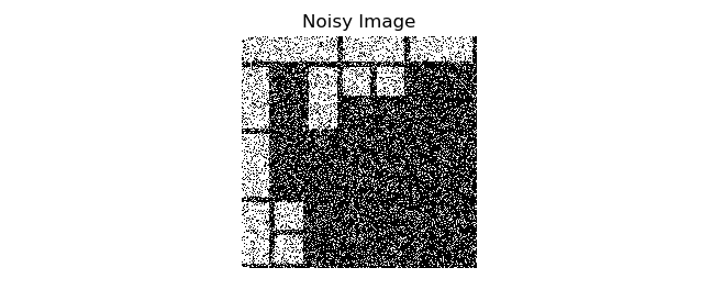
Starting with a black and white Mondrian, I introduced noise by flipping pixels with a probability of .2. The algorithm was run with a non-adaptive stopping criterion of updating every pixel 10 times. Again, the ’true image’ corresponds to \(Y\), the ’noisy image’ to \(X\) and the ‘denoised image’ to \(\hat{Y}\).

You can find corresponding code in my repo.

[0] I did try to rephrase this sentence. ↩