Invitations

Posted on Mar 2, 2020

Scenario and goal

You are the host of an event for which there are $n$ candidates to be invited and you possess sufficient resources to host all candidates. Let the nature of the event be such that it seems personally attached to you, yet also fairly polarizing in its experience. In other words:

some invitees will have a desire to decline
invitees with a desire to decline will feel bad about declining
some non-invitees will have a desire to attend
non-invitees with a desire to attend will feel bad about not being able to attend

Moreover, one might weigh the ambitions wrt non-desiring invitees and desiring non-invitees differently. For instance, one might consider the discomfort of someone having to decline, and thereby expressing his/her lack of appreciation, worse than the missed opportunity of someone not attending who would’ve desired to.

Concretely, this gives rise to the goal of minimizing the following quantities:

non-desiring invitees
desiring non-invitees

Thus, recalling the option to weigh those terms differently, we obtain the following loss function: \[\mathcal{L} := \alpha \cdot \text{\#non-desiring invitees} + (1 - \alpha) \cdot \text{\#desiring non-invitees}\] with $\alpha \in [0, 1]$.

If we had perfect a priori knowledge about candidates desires and would either invite according to it or its negation, our loss function would evaluate to $0$ or $n$ respectively. As those represent ‘best’ and ‘worst’ cases, we can set our expectation of algorithm performance to be within the range $[0, n]$.

Assumptions

Candidate desires to attend the event are i.i.d. with $\Pr[\text{desire}] = q$.
$q$ is unknown.
Invitation candidates respond to the invitation according to their desire.

Algorithms and their performances

Let’s start off with some naive deterministic algorithms before we delve into randomized approaches.

Naive 1: Invite all candidates

$$\begin{aligned} \mathbb{E}[\mathcal{L}] &= \alpha \mathbb{E}[\text{\#non-desiring candidates}]\\ &= \alpha n (1-q) \end{aligned}$$

Naive 2: Invite nobody

$$\begin{aligned} \mathbb{E}[\mathcal{L}] &= (1 - \alpha) \mathbb{E}[\text{\#desiring candidates}] \\ &= (1 - \alpha)n q \end{aligned}$$

Randomized 1: Invite candidates i.i.d. with $\Pr[\text{invite}]=p$

$$\begin{aligned} \mathbb{E}[\mathcal{L}] &= \alpha \mathbb{E}[\text{\#non-desiring candidates}] \Pr[\text{invite}] + (1 - \alpha) \mathbb{E}[\text{\#desiring candidates}] \Pr[\text{no invite}] \\ &= \alpha n (1 - q) p + (1 - \alpha)n q (1 - p) \end{aligned}$$

Naturally, one might wonder what shape the optimal $p$ takes on, as a function of $\alpha$ and $q$.

$$\begin{aligned} \hat{p} :&= argmin_{p}\ \mathcal{L} \\ &= argmin_{p}\ \alpha n (1 - q) p + (1 - \alpha)n q (1 - p) \\ &= argmin_{p}\ p (\alpha (1 - q) + (1 - \alpha)q(-1)) \\ &= argmin_{p}\ p (\alpha - q) \end{aligned}$$

Recalling that $p$ is a probability, we know it is bounded by $[0, 1] $. Hence there are three cases:

$\hat{p} := 0$ if $\alpha > q$
$\hat{p} := 1$ if $\alpha < q$
$p$ is irrelevant if $q = \alpha$

What does this tell us? In the first case, we would like to go with the naive ‘invite nobody’ approach whereas in the second case, we would like to go with the ‘invite everybody’ approach. Intuitively this might come as a slight surprise - why aren’t there any cases in which the optimal $p$ lies inbetween $0$ and $1$, after all? I think the route towards insight as to why this doesn’t happen is to emphasize that all candidates are drawn i.i.d. with $p$.

However, as $q$ is assumed to be unknown, we cannot evaluate said condition. In other words, depending on $\alpha$ and $q$, one of Naive 1 and Naive 2 will perform well, the other badly. This randomized approach will lie somewhere in-between. Allowing for an adaptive approach, i.e. letting $p$ vary over time, we could ‘push’ $p$ closer to either $0$ or $1$, whichever is preferable. Such a method would naturally end up with a loss between that of the fixed starting probability $p$ and the approached ‘invite all’ or ‘invite nobody’ approach. For instance, if asking everybody is the optimal choice, the relative ordering of expected losses looks as follows:

losses

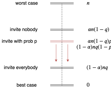
The red arrows indicate the direction in which we’d like to shift the randomized approach by making it adaptive.

Note that in order to devise an adaptive strategy, we need to consecutively sample feedback. Hence candidates invitations are no longer i.i.d. but rather invited one after another, each possibly influencing all of the remaining candidates.

Randomized 2: Update invitation propabilities $p_i$

Given a $p$ such that $p_1 = p$ and $\delta > 0$.

for i = 1 to n:
    invite candidate i with probability p_i
    if candidate i was invited:
        if candidate i accepts:
           p_{i+1} := p_i + delta
        else:
           p_{i+1} := p_i - delta

We assume that $delta$ is small enough such that $[0, 1] \subset [p_1 - n \delta; p_1 + n \delta]$. If not, one could simply cut $p_i$ off at 0 and 1 respectively.

In order to analyze the expected loss of this approach, it turns out useful to ask another question first: How many candidates will be invited with this approach?

The iterative process of updating $p_i$ can be thought of as a random walk on the following Markov chain:

probability updates

By definition, the likelihood of candidate $i$ receiving an invitation depends on the state we find ourselves in in timestep $i$. Referring to a state and its associated value $p_i$ by $S_i$, our question of the total amount of invitees translates to:

\[\mathbb{E}[\text{\#invitees}] = \mathbb{E}[\sum_{i=1}^n S_i]\]

Before addressing the evaluation of this quantity, we first derive a helpful notion: the expected state in timestep $i$. $$\begin{aligned} \mathbb{E}[S_i] &= \mathbb{E}[p_1 + \delta \cdot \text{\#‘right’ transitions so far} - \delta \cdot \text{\#’left’ transitions so far}]\\ &= p_1 + \delta \cdot \mathbb{E}[\text{\#‘right’ transitions so far}] - \delta \cdot \mathbb{E}[\text{\#’left’ transitions so far}] \text{ (L.O.E.)}\\ &= p_1 + \delta (i-1)q - \delta(i-1)(1-q) \end{aligned}$$

Coming back to our underlying question, we obtain: $$\begin{aligned} \mathbb{E}[\text{\#invitees}] &= \mathbb{E}[\sum_{i=1}^n S_i] \\ &= \sum_{i=1}^n \mathbb{E}[S_i] \text{ (L.O.E.)} \\ &= \sum_{i=1}^n p_1 + \delta (i-1)q - \delta(i-1)(1-q) \\ &= n p_1 + \delta \frac{n(n-1)}{2}(2q - 1) \\ &= n (p_1 + \delta \frac{n-1}{2}(2q - 1)) \end{aligned}$$

For the sake of compactness, let us define $r := p_1 + \delta \frac{n-1}{2}(2q - 1)$. Plugging this into our loss function, we learn that:

… so did we really improve on the first randomized, non-adaptive approach, with fixed $p$? A closer examination of $r$ yields the insight. We see that $r < p_1$ if $q < \frac{1}{2}$ and $r > p_1$ if $q > \frac{1}{2}$. In other words, this approach is an enhancement over the former if either is satisfied:

$\alpha > q$ and $\frac{1}{2} > q$
$\alpha < q$ and $\frac{1}{2} < q$.

On the one hand, it might seem like a disappointment that it is not always an improvement over the randomized approach with fixed probability. On the other hand, we now see (more clearly) why such hopes were unfounded: Our update rule is independent of $\alpha$. Yet, $\alpha$ determines the loss function. An alternative approach, paving the way towards strict superiority and leveraging $\alpha$ in the update step seems very feasible, albeit possibly less simple and clean. :)

Furthermore, note that the dependence of $r$ on $n$ implies that given the satisfaction of either condition, the loss of this approach converges towards the loss of optimal fixed $p$ with increasing number of candidates, $n$.

Closing remarks

It seems to me that what we are doing in the update step can be seen as implicitly maintaining and leveraging a counter on the binary outcomes of desire preferences. This is a flavor of explore-exploit.
The addition of $\delta$s in the update step is a design choice. Multiplication seems like a sensible approach, too.
$\delta$ is a hyperparameter.
Many thanks to Tim and Daan.